
Chemostat DDE-ESA
Chemostat DDE-ESA: Documentation
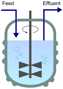
Stirred bioreactor operated as a chemostat, with continuous inflow (Feed) and outflow (Effluent).
Table of Contents
1. Chemostat
A chemostat (from "Chemical environment is static") is a bioreactor to which fresh medium with nutrient (substrate) is continuously added, while culture liquid is continuously removed to keep the culture volume constant. By changing the rate at which medium is added to the bioreactor the growth rate of the culture (microorganism) can be easily controlled [Wiki-Chemostat].
2. Delay Differential Equations (DDE)
Delay differential equations (DDEs) are a type of differential equations in which the derivative of the unknown function at a certain time is given in terms of the values of the function at previous times. The general form of the time-delay differential equation for \(x(t)\) is
where \(x_t=\{x(\tau):\tau\leq t\}\) represents the trajectory of the solution in the past [Wiki-DDE].
3. Mathematical Model
We consider a well-known anaerobic digestion model for biological treatment of wastewater in a continuously stirred tank bioreactor described by four nonlinear ordinary differential equations [2]. We modify the model by introducing discrete time delays in the equations to represent the delay in the conversion of nutrient consumed by the viable biomass.
The DDE system (1):
\(s'_{1}(t)=u\left(s_{1}^{in}-s_{1}(t)\right)-k_{1}\mu_{1}\left(s_{1}(t)\right)x_{1}(t)\)
\(x'_{1}(t)=e^{-\alpha u \tau_{1}}\mu_{1}\left(s_{1}(t-\tau_{1})\right)x_{1}(t-\tau_{1})-\alpha u x_{1}(t)\)
\(s'_{2}(t)=u\left(s_{2}^{in}-s_{2}(t)\right)+k_{2}\mu_{1}\left(s_{1}(t)\right)x_{1}(t)-k_{3}\mu_{2}\left(s_{2}(t)\right)x_{2}(t)\)
\(x'_{2}(t)=e^{-\alpha u \tau_{2}}\mu_{2}\left(s_{2}(t-\tau_{2})\right)x_{2}(t-\tau_{2})-\alpha u x_{2}(t)\)
with gaseous output
The state variables \(s_1\), \(s_2\), \(x_1\) and \(x_2\) denote substrate and biomass concentrations, respectively: \(s_1\) is the organic substrate, characterized by its chemical oxygen demand (COD), \(s_2\) denotes the volatile fatty acids (VFA), \(x_1\) and \(x_2\) are the acidogenic and methanogenic bacteria respectively; \(s_1^{in}\) and \(s_2^{in}\) are the input substrate concentrations. The parameter \(\alpha \in (0,1)\) represents the proportion of bacteria that are affected by the dilution rate \(u\). The constants \(k_1\), \(k_2\) and \(k_3\) are yield coefficients related to COD degradation, VFA production and VFA consumption respectively.
The constants \(\tau_j\ge 0\), \(j=1,2\), stand for the time delay in conversion of the corresponding substrate to viable biomass for the j-th bacterial population. The terms \(\displaystyle e^{- \alpha u \tau_j}x_j (t-\tau_j)\), represent the biomass of those microorganisms that consume nutrient \(\tau_j\) units of time prior to time \(t\) and that survive in the chemostat the \(\tau_j\) units of time necessary to complete the process of converting the nutrient to viable biomass at time \(t\).
The functions \(\mu_1(s_1)\) and \(\mu_2(s_2)\) model the specific growth rates of the bacteria \(x_1\) and \(x_2\) respectively. The output \(Q\) describes the methane (biogas) flow rate, where \(k_4\) as a yield coefficient.
4. Asymptotic stability of the model solutions
In [3] we prove in Theorem 1 that there exists a suitable upper bound \(u_b>0\) of \(u\) such that for any (admissible) value of the dilution rate \(u \in (0, u_b)\) there exists an equilibrium point which is globally asymptotically stable for the system (1).
It is interesting to note that the qualitative behavior of the solutions of the system (1) with \(\tau_1>0\), \(\tau_2>0\) is the same as the solutions behavior of the model without delays, i. e. when \(\tau_1=\tau_2=0\).
5. Maximizing the Biogas Production
Denote by \(u \in (0, u_b)\) some value of the dilution rate and consider the equilibrium point \(p(u) = (s_1(u), x_1(u), s_2(u), x_2(u))\). Denote further by
the output, defined on the set of all steady states \(p(u)\), parameterized on \(u\). \(Q(u)\) is called input-output static characteristic of the model.
Assume that the function \(u \to Q(u)\), \(u \in (0, u_b)\), is strictly unimodal, i.e. there exists a unique point \(u_{\max} \in (0, u_b)\) where Q(u) takes a maximum.
Denote further \(p(u_{\max}) = (s_1(u_{\max}), x_1(u_{\max}), s_2(u_{\max}), x_2(u_{\max})).\) Our goal is to stabilize the system (1) towards the (unknown) equilibrium point \(p(u_{\max})\) and therefore to the maximum methane flow rate \(Q_{\max}\). This is realized by applying a numerical model-based extremum seeking algorithm (ESA) in accordance with the assumption and the requirements of Theorem 1.
The main idea of the algorithm is the following: we construct a sequence of points \(u^{(1)}, u^{(2)}, \ldots, u^{(n)}, \ldots\) from the interval \((0,u_b)\), each \(u^{(j)}\) being in the form \(u^{(j)} = u^{(j-1)} \pm h\), \(h>0\), and such that the sequence \(\{u^{(j)}\}\) tends to \(u_{\max}\); Theorem 1 guarantees that the dynamics is globally asymptotically stabilizable towards the equilibrium \(p(u^{(j)})\), \(j=1,2,\ldots\). Then by computing and comparing the values \(Q(p(u^{(1)})), Q(p(u^{(2)})), \ldots, Q(p(u^{(n)})), \ldots \) and thus \(Q_{\max}\) are achieved.
In the computer implementation the algorithm is carried out in two stages. In Stage I, "rough" intervals \({[}U{]}\) and \({[}Q{]}\) are found which enclose \(u_{\max}\) and \(Q_{\max}\) respectively; in Stage II, the interval \({[}U{]}\) is refined using an elimination procedure based on the golden mean value (or Fibonacci search) strategy. Stage II produces the final intervals \({[}u_{\max}{]} = {[}u_{\max}^{-}, u_{\max}^{+}{]}\) and \({[}Q_{\max}{]}\) such that \(u_{\max} \in {[}u_{\max}{]}\), \(Q_{\max} \in {[}Q_{\max}{]}\) and \((u_{\max}^{+} - u_{\max}^{-}) \leq \epsilon\), where the tolerance \(\epsilon >0\) is specified by the user.
6. Computer simulation
The following specific growth rate functions are considered in the model:
In the simulation process we use the following numerical values for the model coefficients, which are obtained by real experiments [1]:
To demonstrate the extremum seeking algorithm we consider the discrete delays \(\tau_1=2\) and \(\tau_2=7\). The initial conditions are \(\varphi_{s_1}(t) =2\), \(\varphi_{x_1}(t)=0.1\) for \(t \in [-\tau_1, 0]\), and \(\varphi_{s_2}(t)= 10\), \(\varphi_{x_2}(t)=0.05\) for \(t \in [-\tau_2, 0]\).
The numerical outputs are visualized in Figures:
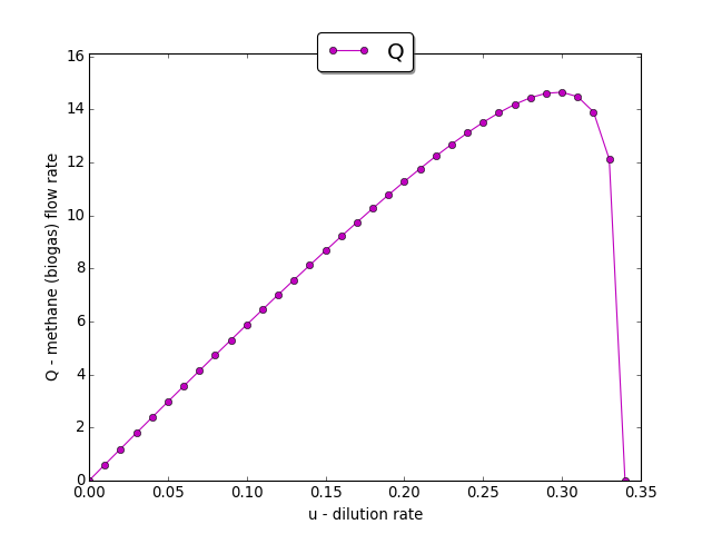
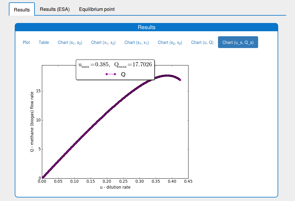
The input-output static characteristic \(Q(u)\)
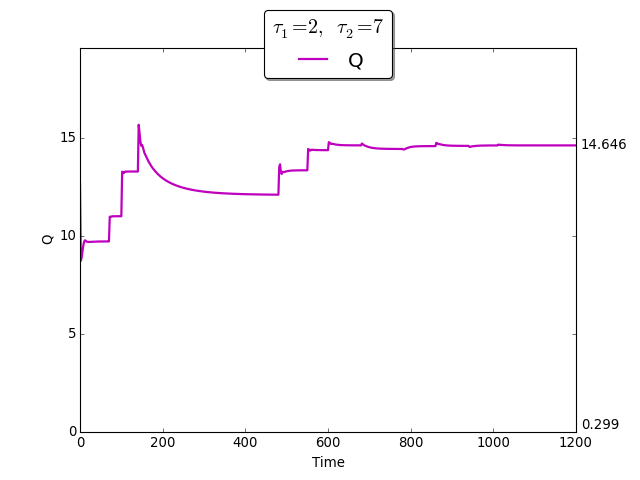
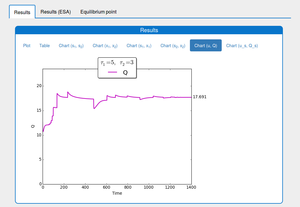
The time evolution of \(Q(t)\) towards \(Q_{\max}\)
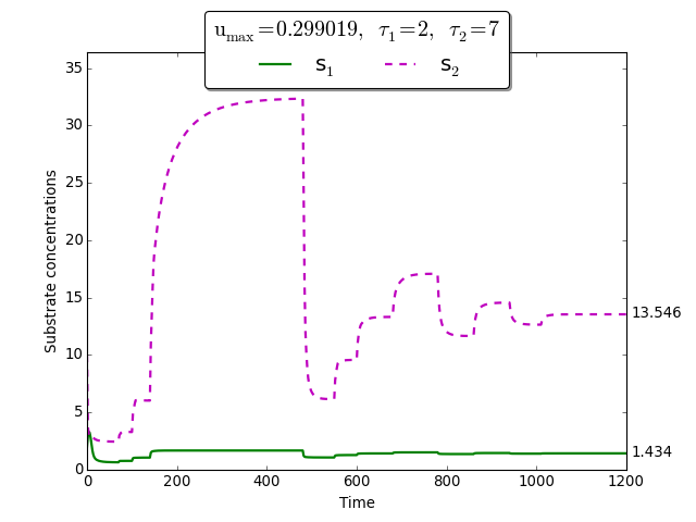
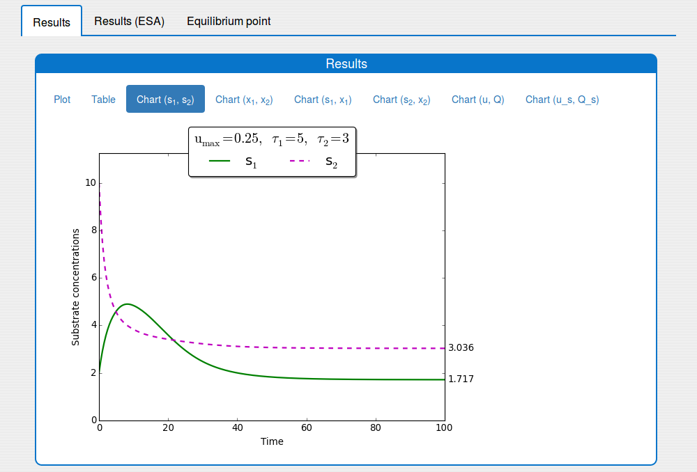
Time evolution of \(s_1(t)\), \(s_2(t)\) towards \(s_1^{\max}\), \(s_2^{\max}\)
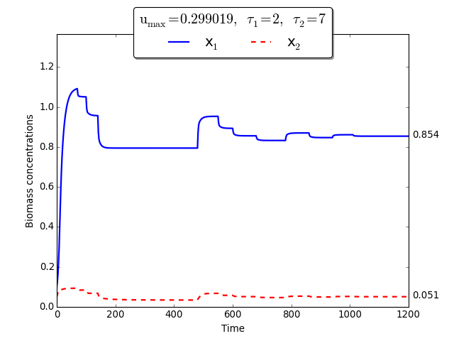
Time evolution of \(x_1(t)\), \(x_2(t)\) towards \(x_1^{\max}\), \(x_2^{\max}\)
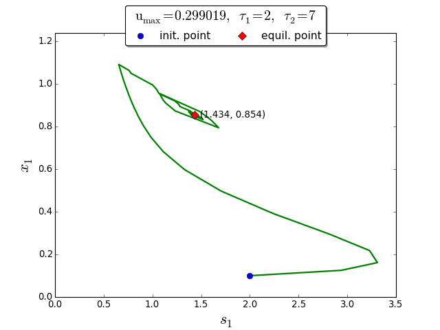
Trajectories in the \((s_1, x_1)\) phase plane
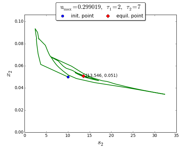
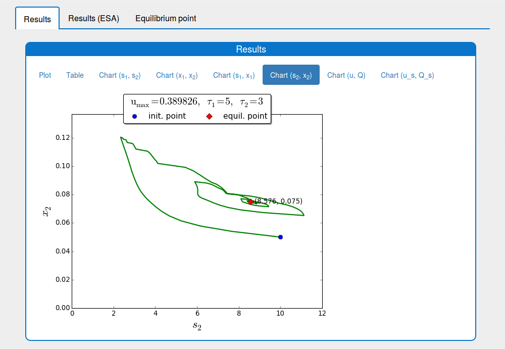
Trajectories in the \((s_2, x_2)\) phase plane
7. References
| [1] | Alcaraz-Gonzalez, et al.: Software sensors for highly uncertain WWTPs: a new apprach based on interval observers}, Water Research 36, 2515--2524 (2002). |
| [2] | Bernard, O., Hadj-Sadok, Z., Dochain, D., Genovesi, A., Steyer, J.-P.: Dynamical model development and parameter identifcation for an anaerobic wastewater treatment process. Biotechnology and Bioengineering 75, 424–438 (2001). |
| [3] | Milen K. Borisov, Neli S. Dimitrova, Mikhail I. Krastanov: Global Asymptotic Stability of a Functional Differential Model with Time Delay of an Anaerobic Biodegradation Process. To appear in Serdica Journal of Computing, 2017. |
| [Wiki-Chemostat] | http://en.wikipedia.org/wiki/Chemostat |
| [Wiki-DDE] | http://en.wikipedia.org/wiki/Delay_differential_equation |
8. Acknowledgements
This work has been supported by the Bulgarian Academy of Sciences, Programme for Support of Young Scientists and Scholars, grant No. DFNP-88/04.05.2016.
Chemostat DDE-ESA: User Manual
Stirred bioreactor operated as a chemostat, with continuous inflow (Feed) and outflow (Effluent).
Table of Contents
1. User Interface
The user interface (UI) of the application is divided on three parts:
1.1. Inputs
In the 'Inputs' part the user can:
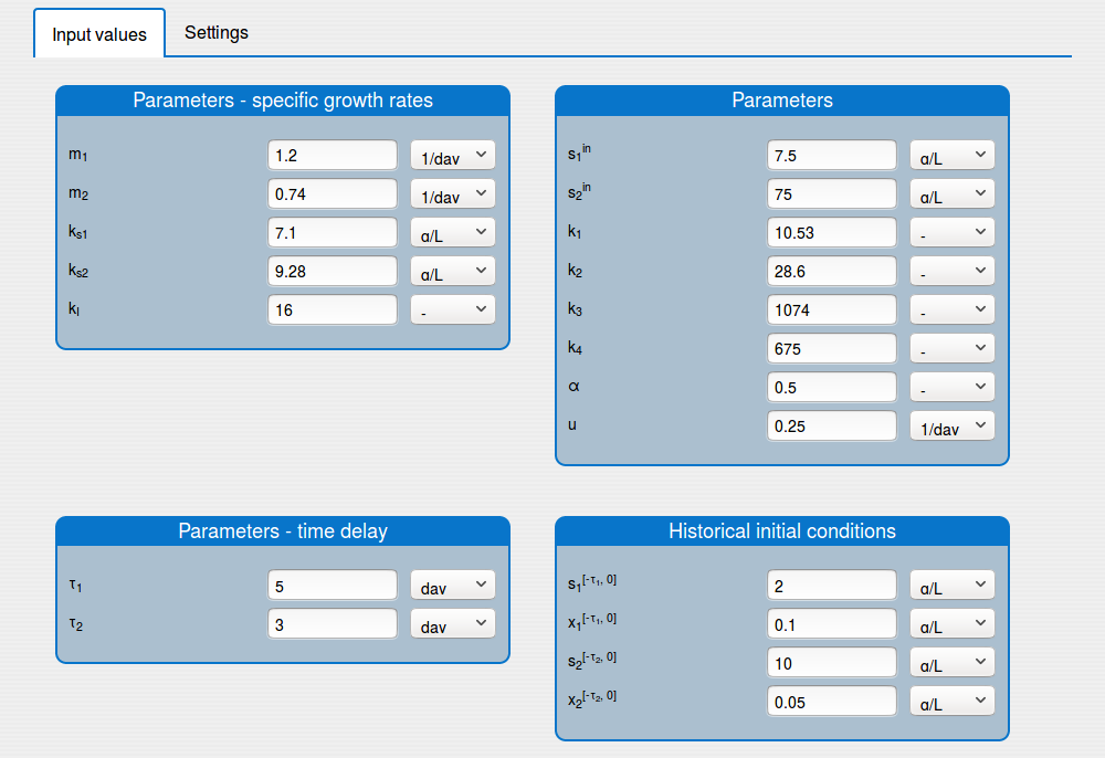
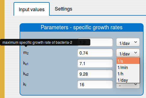
set the values of the parameters of the system (see the tab 'Input values');
set the initial conditions of the system (see the tab 'Input values');
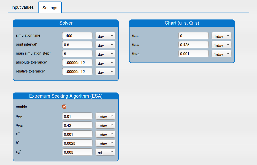
set up the solver's settings (see the tab 'Settings');
enable/disable the extremum seeking algorithm (see the tab 'Settings').
1.2. Buttons
This UI part contains the buttons:
- 'Compute' button runs the simulation;
- 'Save' button saves the inputs values on the server or on a local file (e.g. xxx.dat);
- 'Load' button loads the local file with the input values

1.3. Outputs
The 'Outputs' part shows the results of the simulation:
'Results' tab shows the results in:
- an interactive plot (see the tab 'Results/Plot')
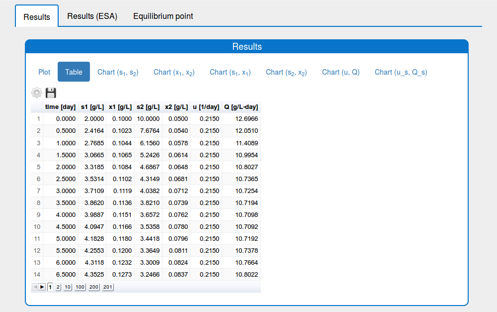
- a table format (see the tab 'Results/Table')
- static images (see the tabs 'Results/Chart (s1,s2)', ... , 'Results/Chart (u_s, Q_s)');
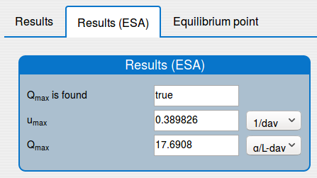
'Results (ESA)' tab shows the results of applying the extremum seeking algorithm to the system (1);
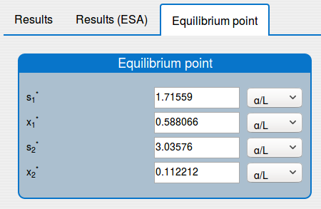
'Equilibrium point' tab shows the results of the equilibrium point computation.
2. How to Do?
The application can:
- compute \(u_{max}\) and \(Q_{max}\) respectively
- compute the equilibrium point of the system (1), see the 'Chemostat DDE-ESA (Doc)';
- simulate the system;
- apply the extremum seeking algorithm to the system;
2.1. How to compute \(u_{max}\) and \(Q_{max}\)?
Steps:
Enter the values for the input parameters and the historical initial conditions of the system in the tab 'Inputs/Input values'.
Note. The parameter \(u\) (dilution rate) is not used.
Set the values for the min and max dilution rate and the searching step in the box 'Inputs/Settings/Chart (u_s, Q_s)'.
Disable the extremum seeking algorithm in the box 'Inputs/SettingsESA'.
Set the simulation time on 0 in the 'Inputs/Settings/Solver'.
Note. The other solver's settings are not used.
Press 'Compute' button and wait for the result.
See the result in the plot 'Outputs/Results/Chart(u_s,Q_s)':
2.2. How to compute the equilibrium point of the system?
Steps:
Enter the values for the input parameters and the historical initial conditions of the system in the tab 'Inputs/Input values'.
Disable the extremum seeking algorithm in the box 'Inputs/SettingsESA'.
Set the simulation time on 0 in the 'Inputs/Settings/Solver'.
Note. The other solver's settings are not used.
Press 'Compute' button and wait for the result.
See the result in the tab 'Outputs/Equilibrium point":
2.3. How to simulate the system?
Steps:
Enter the values for the input parameters and the historical initial conditions of the system in the tab 'Inputs/Input values'.
Disable the extremum seeking algorithm in the box 'Inputs/SettingsESA'.
Set on the solver's settings in the 'Inputs/Settings/Solver'.
Notes:
- The 'print interval' should be 1/10 from the 'main simulation step'.
- The 'simulation time' should be multiples of the 'main simulation step'
Press 'Compute' button and wait for the result.
See the result in the tab 'Outputs/Results" and sub-tabs: 'Plot', 'Table', ..., 'Chart(u,Q)`:
2.4. How to apply the extremum seeking algorithm to the system?
Steps:
Enter the values for the input parameters and the historical initial conditions of the system in the tab 'Inputs/Input values'.
Note. The parameter \(u\) (dilution rate) is not used.
Enable the extremum seeking algorithm in the box 'Inputs/SettingsESA'.
Set on the solver's settings in the 'Inputs/Settings/Solver'.
Notes:
- The 'print interval' should be 1/10 from the 'main simulation step'.
- The 'simulation time' should be multiples of the 'main simulation step'
Press 'Compute' button and wait for the result.
See the result in the tab 'Outputs/Results" and sub-tabs: 'Plot', 'Table', ..., 'Chart(u,Q)`:
3. Features
There are some UI features:
In the 'Inputs' part:
a short description (tooltip) for most of the input parameters;
a possibility to change the unit of the input parameters and variables;
In the 'Results/Plot' tab it is possible to:
save the current state of the plot in the png image (click 'Save' icon);
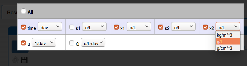
show/hide plot's variables (click 'Settings' icon);
change the unit of some plot variable (click 'Settings' icon);
zoom in the plot (use the mouse horizontal or vertical drag);
return the plot to the initial zoom (double click with the mouse);
see the values of the variables

4. Acknowledgements
This work has been supported by the Bulgarian Academy of Sciences, Programme for Support of Young Scientists and Scholars, grant No. DFNP-88/04.05.2016.