
Pipe Flow

Pipe Flow
Pipe parameters
1. Parameters
| Symbol | Parameter name | Unit |
|---|---|---|
| \(d_i\) | internal pipe diameter | mm |
| \(d_e\) | external pipe diameter | mm |
| \(L\) | pipe length | m |
| \(\varepsilon\) | pipe surface roughness | mm |
| \(p_i\) | inlet pressure | bar |
| \(T_i\) | inlet temperature | K |
| \(\dot{m}\) | inlet mass flow rate | kg/h |
| \(T_w\) | pipe temperature | K |
2. Geometry properties
The flow area is:
The fluid volume is:
The internal and external surface areas are calculated as:
The mass of the pipe is:
where \(\rho_p\) is the density of the pipe material (steel, aluminum etc.)
3. Pressure losses
In general the pressure loss in pipes and components depends on the upstream fluid density \(\rho\) and the flow velocity
This pressure loss can be calculated from the formula:
where \(c_{d}\) is the flow drag coefficient. For pipes the drag coefficient depends on the pipe geometry and the Darcy friction factor \(\zeta\) [Wikip-DFF]:
where \(L\) is the length of the pipe and \(d_i\) is the internal diameter of the pipe.
The friction factor depends on the Reynolds number \(Re={\rho v d}/{\mu}\) and the relative surface roughness \(\varepsilon/d\). It can be determined using the Moody chart
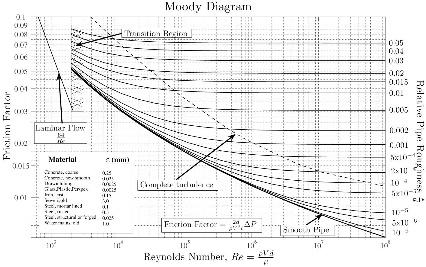
Moody chart
In the laminar region the friction factor depends only on the Reynolds number:
In the turbulent region the relation is more complex and is given by the Colebrook equation [Colebrook39]:
In the limit of high Reynolds numbers the friction factor depends solely on the relative surface roughness.
As the Colebrook correlation is implicit in \(\zeta\), it is not suitable for direct calculations. Different approximations have been developed amongst which special attention deserves the Churchill correlation [Church77], which covers all flow regimes: laminar, transitional and turbulent:
4. Heat Exchange
Heat exchange can be computed with or without iteration. The steps of the algorithm are:
if we have \(Re\), we can find \(Nu=f\left(Re,Pr\right)\) as follows:
- if \(Re<=2300\), the flow is laminar and \(Nu=3.66\)
- for \(1e4<=Re<=1e6\), the flow is turbulent and the Nusselt number is calculated as [VDI]
\begin{equation*} Nu=\frac{\left(\xi/8\right)Re\cdot Pr}{1+12.7\sqrt{\xi/8}\left(Pr^{\frac{2}{3}}-1\right)} \end{equation*}\begin{equation*} \xi=\left(1.8\cdot\log_{10}Re-1.5\right)^{-2} \end{equation*}- the transition range is for \(2300<Re<1e4\), in which the value of \(Nu\) is obtained through linear interpolation
- \(Re>1e6\) are values outside the range of validity
from \(Nu\) the convection coefficient \(\alpha\) is found as
\begin{equation*} \alpha=\frac{\lambda\cdot Nu}{d_{i}} \end{equation*}where \(\lambda\) is the thermal conductivity of the fluid
the heat flow rate is thus
\begin{equation*} \dot{Q}_{w}=\alpha A \Delta T \end{equation*}where \(\Delta T\) is the temperature difference
from
\begin{equation*} \dot{Q}_{w}=\dot{m}\cdot h_i-\dot{m}\cdot h_o \end{equation*}we find the outlet enthalpy \(h_o\) and obtain the value of the outlet temperature \(T_o\) from the fluid state determined by the outlet pressure \(p_o\) and \(h_o\)
In the case of computation with iteration, we guess \(T_o\), compute the fluid properties at mean temperature
and use logarithmic mean temperature difference (LMTD) to caculate the heat exchange:
For computation without iteration, \(\Delta T=T_i-T_w\)
5. References
| [Wikip-DFF] | http://en.wikipedia.org/wiki/Darcy_friction_factor_formulae |
| [Church77] | Churchill, S.W. (November 7, 1977). "Friction-factor equation spans all fluid-flow regimes". Chemical Engineering: 91–92. |
| [Colebrook39] | Colebrook, C.F. (February 1939). "Turbulent flow in pipes, with particular reference to the transition region between smooth and rough pipe laws". Journal of the Institution of Civil Engineers (London). |
| [VDI] | VDI (Verein Deutscher Ingenieure), Heat Atlas, Springer-Verlag, 2010, Part G1: Heat Transfer in Pipe Flow, p.697, eq(26) and (27) |