
Fermantation DDE-ESA
Fermentation DDE-ESA: Documentation
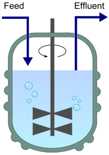
Stirred bioreactor operated as a chemostat, with continuous inflow (Feed) and outflow (Effluent).
Table of Contents
1. Chemostat
A chemostat (from "Chemical environment is static") is a bioreactor to which fresh medium with nutrient (substrate) is continuously added, while culture liquid is continuously removed to keep the culture volume constant. By changing the rate at which medium is added to the bioreactor the growth rate of the culture (microorganism) can be easily controlled [Wiki-Chemostat].
2. Delay Differential Equations (DDE)
Delay differential equations (DDEs) are a type of differential equations in which the derivative of the unknown function at a certain time is given in terms of the values of the function at previous times. The general form of the time-delay differential equation for \(x(t)\) is
where \(x_t=\{x(\tau):\tau\leq t\}\) represents the trajectory of the solution in the past [Wiki-DDE].
3. Mathematical Model
We consider one of the bench-mark mathematical models of the continuous methane fermentation, the so-called "single biomass/single substrate" model. It is described by two nonlinear ordinary differential equations:
and one algebraic equation, presenting the gaseous output (methane):
The state variables \(x=x(t)\) and \(s=s(t)\) represent biomass concentration \([mg/dm^3]\) and substrate concentration \([mg/dm^3]\) respectively, \(s_{in}\) is influent substrate concentration \([mg/dm^3]\), \(u\) is dilution rate \([day^{-1}]\), \(k_1\) is yield coefficient, \(k_2\) is coefficient \([(dm^3)^2/mg]\), and \(Q\) is methane gas flow rate \([dm^3/day]\). The parameter \(\alpha \in (0,1)\) accounts for the biomass retention. The model function \(\mu(s)\) presents the specific growth rate of the biomass.
4. Assumptions on the model
The theoretical studies of the model (ref{met}) are carried out under several assumptions.
Assumption 1. The function \(\mu\) is defined for \(s \in [0, +\infty)\), \(\mu(0)=0\), \(\mu(s)>0\) for \(s > 0\), and \(\mu(s)\) is continuously differentiable for all \(s \geq 0\).
Assumption 2. Lower bounds \(s_{in}^{-}\) and \(k_2^-\) for the values of \(s_{in}\) and \(k_2\) respectively, and an upper bound \(k_1^+\) for the value of \(k_1\) are known.
Denote \(\beta^- = \frac {k_1^+} {k_2^{-} s_{in}^{-}}\) and consider the following feedback control law:
Obviously, \(\kappa (\cdot) = \beta Q(\cdot)\) holds true. Replacing in the model (1) the dilution rate \(u\) by the feedback \(\kappa (s(t-\tau),x(t-\tau))\), where \(\tau >0\) is a discrete delay, we obtain
Choose some \(\beta \in \left( \beta^{-}, \: +\infty \right)\) and define
Note that \(\bar p_\beta\) is an equilibrium point for (4)--(5), and \(\bar s \in (0,s_{in})\).
Assumption 3. There exist points \(s^-\) and \(s^+\) such that \(s^- < \bar s < s^+ < s_{in}\) and
(i) the function \(\\mu\) is strictly increasing on the interval \((s^-, s^+]\);
(ii) \(\mu(s) < \mu(s^-) < \mu(s_{in})\) for each \(s \in [0,s^-)\);
(iii) there exists \(\varepsilon>0\) such that \(\mu(s^+) < \mu (s)\) for each \(s \in (s^+, s^+ + \varepsilon)\).
Denote \(u^-=\mu (s^-)/\alpha\) and \(u^+=\mu (s^+)/\alpha\). Assumption 3 implies that \(u^- < u^+\).
Assumption 4. Each point from the interval \([u^- , u^+]\) is an admissible value for the control function \(u\).
Denote further \(\bar u= \kappa (\bar s, \bar x )= \mu(\bar s)/\alpha\); obviously \(\bar u \in (u^-, u^+)\) holds true.
5. Stability of the equilibrium points
Denote \(b = b(\beta) = k_1 \bar x \mu(\bar s) \mu^\prime (\bar s)\) and \(d = d(\beta) = \mu(\bar s) \left(\frac{1}{\alpha}\mu(\bar s) - k_1 \bar x \mu^\prime (\bar s)\right)\), which comes from the characteristic equation of (4)--(5) evaluated at \(\bar p_{\beta}\).
Theorem 1. Let the Assumptions A1, A2, A3 and A4 be fulfilled.
(i) If \(b \geq d\) then the equilibrium point \(\bar p_{\beta}\) is locally asymptotically stable for any value of the delay \(\tau>0\).
(ii) If \(b<d\) then there exists \(\tau_0>0\) such that the equilibrium point \(\bar p_{\beta}\) is locally asymptotically stable for all values \(\tau\) such that \(0<\tau < \tau_0\); the equilibrium is locally unstable if \(\tau \geq \tau_0\), and a Hopf bifurcation occurs for \(\tau=\tau_0\).
Denote \(\Omega:=\{\zeta=(s,x): \: s>0, \: x>0 \}\) and let \(\zeta^0=(s^0, x^0) \in \Omega\) be such that \(s(t)= s^0>0\) and \(x(t)= x^0>0\) for each \(t\in [-\tau,0]\). Denote by \(\phi(\cdot, \zeta^0)=(s(\cdot), x(\cdot))\) the solution starting from \(\zeta^0\) of the following closed-loop system \(\Sigma\):
where \(\chi(t)\) is defined in the following way:
Obviously, \(\bar p_{\beta} = (\bar s, \bar x)\) is an equilibrium point of \(\Sigma\), i.e. of (7)--(8).
Theorem 2. Let A1, A2, A3 and A4 be fulfilled. Then there exists \(\bar \tau >0\) such that for each \(\tau\in (0,\bar \tau)\) and for each point \(\zeta^0=(s^0,x^0) \in \Omega\) the solution \(\varphi (t, \zeta^0)\) of \(\Sigma\) has the following property: there exists \(T >0\) such that for each \(t > T\), \(\; \varphi (t, \zeta^0) \in \Omega_{s}:=\{(s,x): s \in [s^-, s^+], x>0\}.\)
Remark 1. It follows from Theorem 2 that the feedback (9) ensures attractivity of the region \(\Omega_s\) independently of the value of the time delay \(\tau \geq 0\). If \(s^-\) and \(s^+\) are sufficiently close to each other, then the trajectories remain close to \(\bar s\) because \(\bar s \in (s^-, s^+)\) holds true. If \(\tau>0\) is sufficiently small, one can easily apply the Lyapunov functions approach to prove that \((s(t), x(t))\) tends to \((\bar s, \bar x)\) as \(t \to \infty\). The existence of \(\Omega_s\) is important for the practical applications (cf. [2]).
Remark 2. The proofs of the two theorems are given in [1].
6. Numerical extremum seeking
Consider the Haldane model function for the specific growth rate
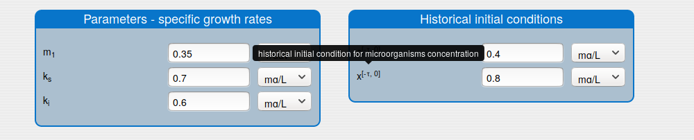
where \(m_1\) is the maximum specific growth rate of the microorganisms \([1/day]\), \(k_s\) and \(k_i\) are the saturation and inhibition constants respectively.
We use the following values for the model coefficients (cf. [3]):
\(k_1 = 3, \; s_{in} = 2, \; m_1=0.35, \; k_s=0.7, \; k_i=0.6, \; \alpha=0.5, \; k_2 = 5.6\).
With \(k_1^{+} = 3.1\) and \(s_{in}^{-} = 1.95\), \(k_2^-=5.59\) we obtain \(\beta^- \approx 0.2844\).
The function \(\mu(s)\) achieves its maximum at the point \(s_{\mu_{\max}} = \sqrt{k_s k_i} \approx 0.6481\) and \(\mu(s)\) is strongly increasing for \(s \in (0, s_{\mu_{\max}})\). Solving the equation \(\bar s = s_{\mu_{\max}}\) with respect to \(\beta\) implies \(\beta = \beta_{\mu_{\max}} \approx 0.3963\). Since \(\bar s\) is an increasing function of \(\beta\), it suffice to consider \(\beta \in (\beta^-, \beta_{\mu_{\max}})\) in order to have Assumption 3 satisfied. For the simulation we also consider \(\beta \in (0.29, 0.39)\) and take \(s^- = 0.1527\), \(u^- = 0.1199\), \(s^+ = 0.6264 < s_{\mu_{\max}}\), \(u^+ = 0.2214\); obviously \(s_{\max} \in (s^-,s^+)\).
For the simulation we also consider \(\beta \in (0.29, 0.39)\) and take \(s^- = 0.1527\), \(u^- = 0.1199\), \(s^+ = 0.6264 < s_{\mu_{\max}}\), \(u^+ = 0.2214\); obviously \(s_{\max} \in (s^-,s^+)\).
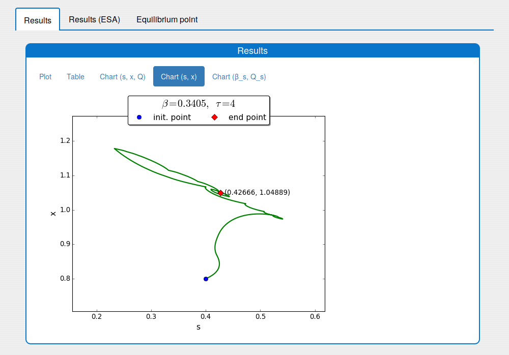
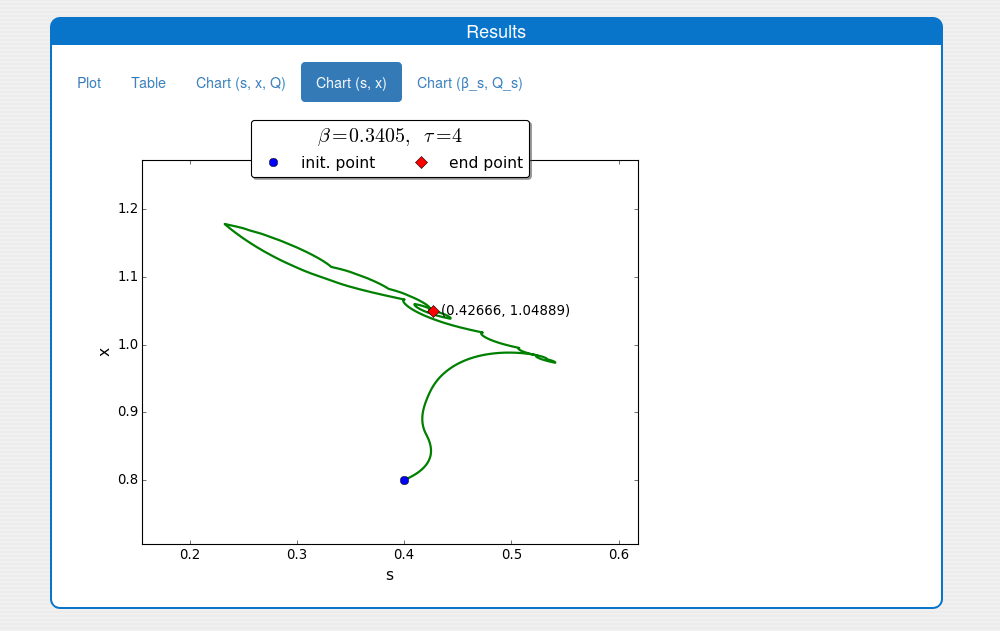
An iterative numerical extremum seeking algorithm (ESA) is applied to \(\Sigma\) aimed to maximize the methane flow rate in real time. The numerical results are visualized in the next figures for \(\tau=4\).
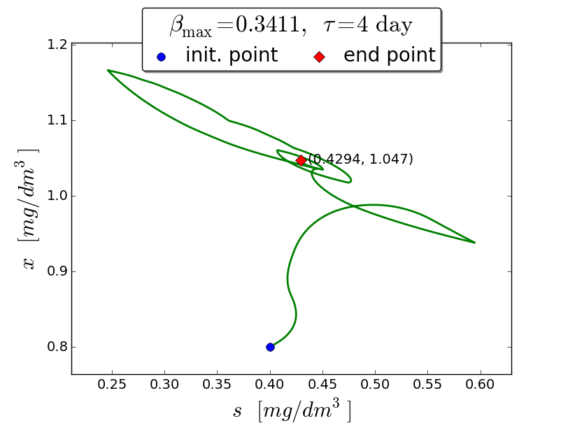
A trajectory in the \((s, x)\) phase plane
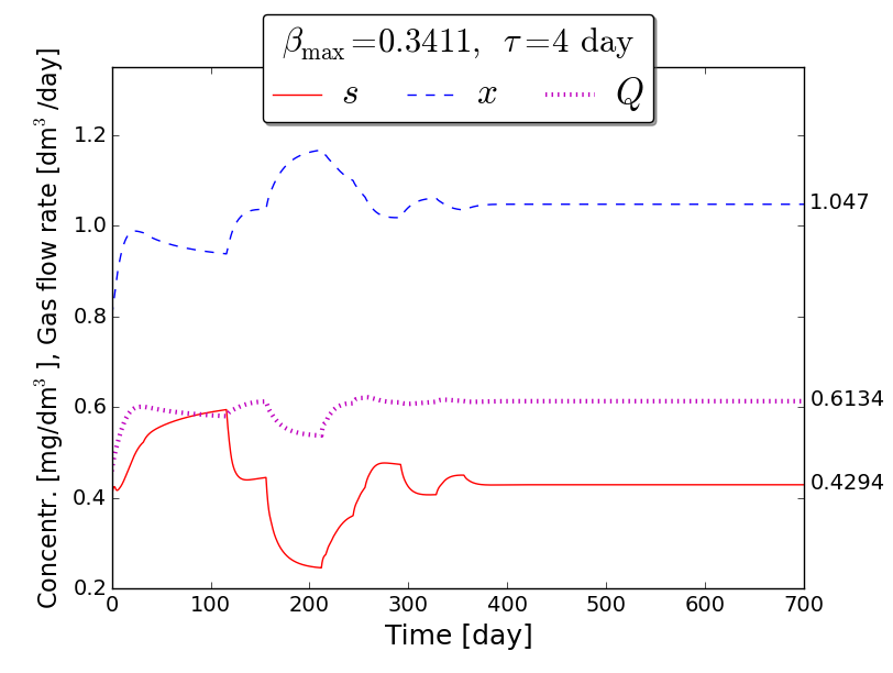
Time evolution of \(s(t)\), \(x(t)\), \(Q(t)\) towards \(s_{\max}\), \(x_{\max}\), \(Q_{\max}\)
7. References
| [1] | Borisov M.K., Dimitrova N.S., Krastanov M.I. (2019) Model-Based Stabilization of a Fermentation Process Using Output Feedback with Discrete Time Delay. In: Nikolov G., Kolkovska N., Georgiev K. (eds) Numerical Methods and Applications (NMA 2018), Lecture Notes in Computer Science, Springer, vol. 11189, 342–350, 2019. ISBN 978-3-030-10692-8 |
| [2] | Grognard, F., Bernard, O.: Stability analysis of a wastewater treatment plant with saturated control. Water Sci Technol 53 (1), 149--157 (2006). |
| [3] | Simeonov I., Mathematical modeling and parameters estimation of anaerobic fermentation process, Bioprocess Engineering, 21 (4), 377--381 (1999). |
| [Wiki-Chemostat] | http://en.wikipedia.org/wiki/Chemostat |
| [Wiki-DDE] | http://en.wikipedia.org/wiki/Delay_differential_equation |
8. Acknowledgements
The work of the first and the second author has been partially supported by the Bulgarian Academy of Sciences, the Program for Support of Young Scientists and Scholars, grant No. DFNP-17-25/25.07.2017. The work of the third author has been partially supported by the Sofia University “St. Kl. Ohridski” under contract No. 80-10-133/25.04.2018.
Fermentation DDE-ESA: User Manual
Stirred bioreactor operated as a chemostat, with continuous inflow (Feed) and outflow (Effluent).
Table of Contents
1. User Interface
The user interface (UI) of the application is divided on three parts:
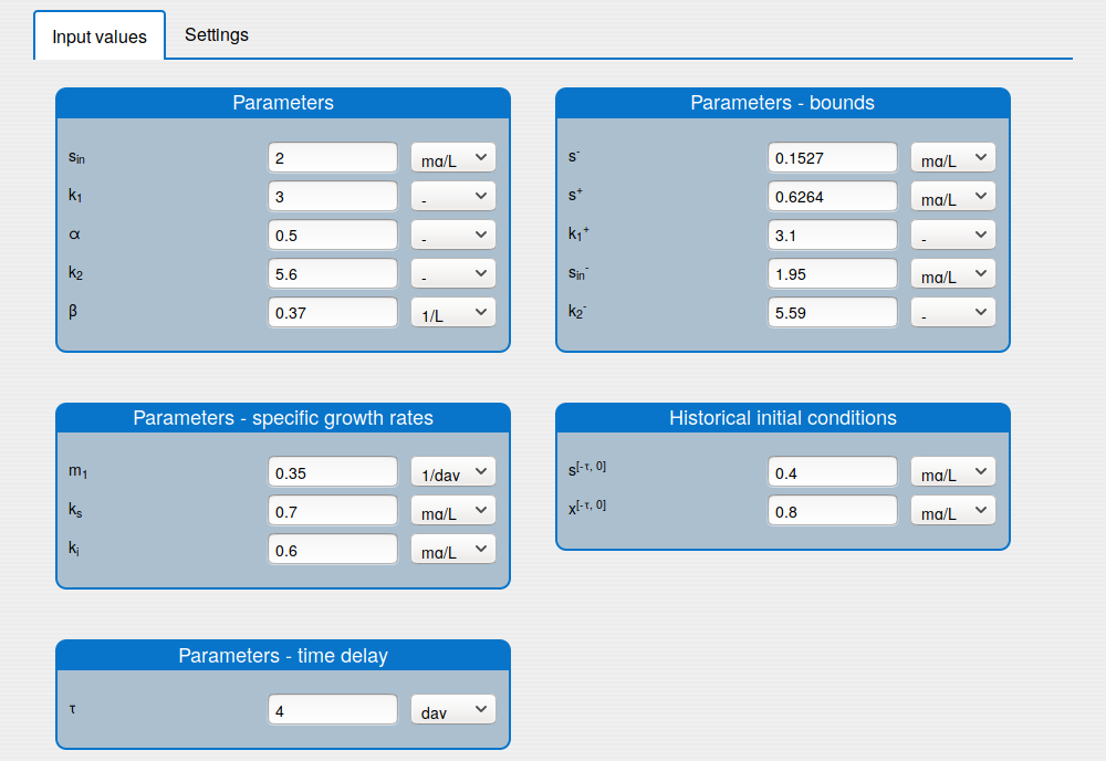
1.1. Inputs
In the 'Inputs' part the user can:
set the values of the parameters (see the tab 'Input values');
set the historical initial conditions (see the tab 'Input values');
set up the solver's settings (see the tab 'Settings');
enable/disable the extremum seeking algorithm (see the tab 'Settings').
1.2. Buttons
This UI part contains the buttons:
- 'Compute' button runs the simulation;
- 'Save' button saves the inputs values on the server or on a local file (e.g. xxx.dat);
- 'Load' button loads the local file with the input values

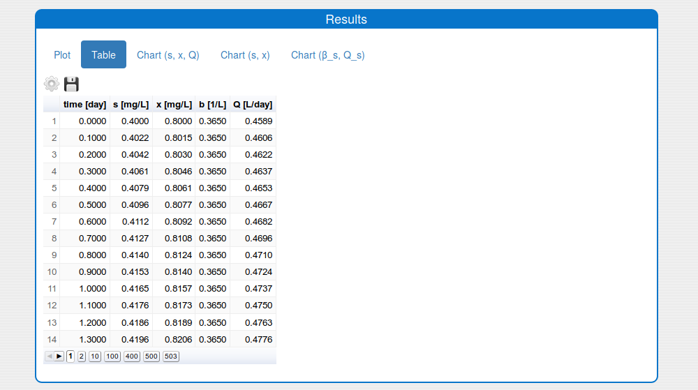
1.3. Outputs
The 'Outputs' part shows the results of the simulation:
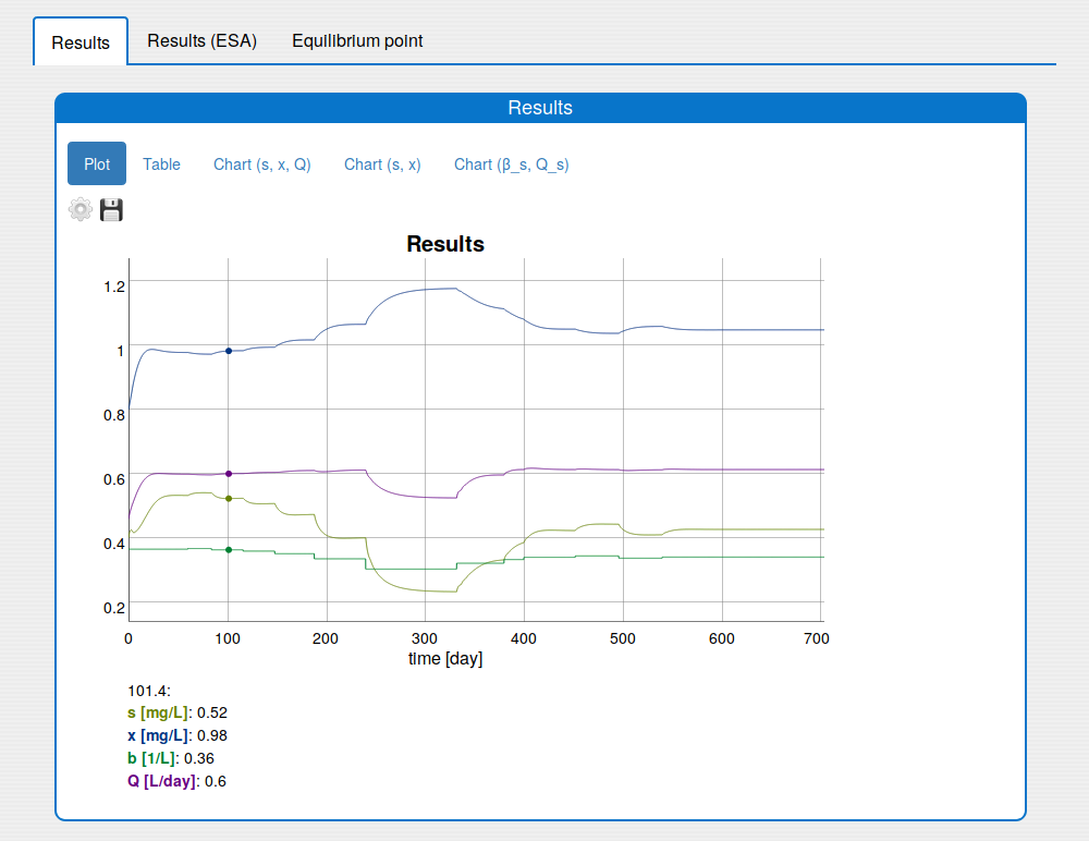
'Results' tab shows the results in:
- an interactive plot (see the tab 'Results/Plot')
- a table format (see the tab 'Results/Table')
- static images (see the tabs 'Results/Chart (s, x, Q)', 'Results/Chart (s,x)' and 'Results/Chart (b_s, Q_s)');
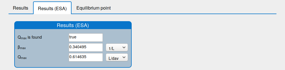
'Results (ESA)' tab shows the results of applying the extremum seeking algorithm to the system (1);
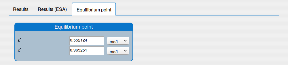
'Equilibrium point' tab shows the results of the equilibrium point computation.
2. How To Do?
The application can:
- compute \(\beta_{max}\) and \(Q_{max}\) respectively
- compute the equilibrium point of the system (1), see the 'Chemostat DDE-ESA (Doc)';
- simulate the system;
- apply the extremum seeking algorithm to the system;
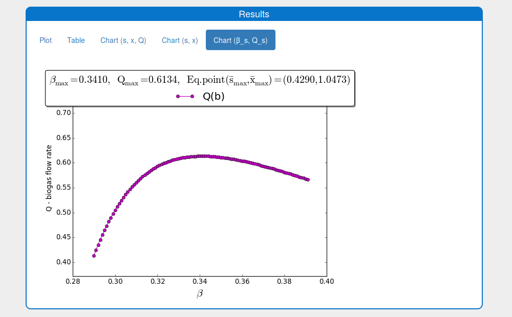
2.1. How to compute \(\beta_{max}\) and \(Q_{max}\)?
Steps:
Enter the values for the input parameters and the historical initial conditions of the system in the tab 'Inputs/Input values'.
Note. The parameter \(\beta\) is not used.
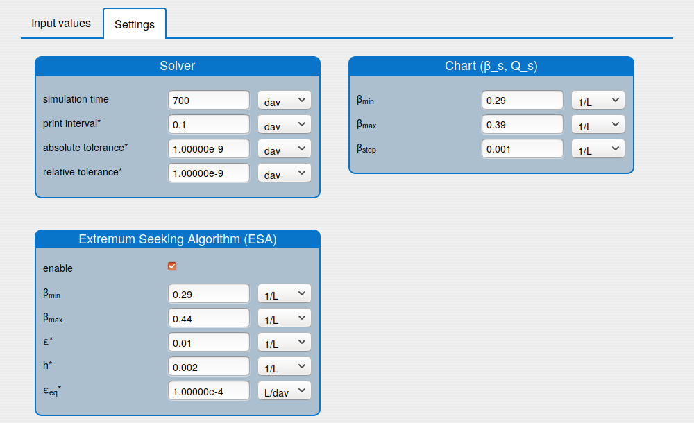
Set the values for the min and max \(\beta\) and the searching step in the box 'Inputs/Settings/Chart (b_s, Q_s)'.
Disable the extremum seeking algorithm in the box 'Inputs/Settings/ESA'.
Set the simulation time on 0 in the 'Inputs/Settings/Solver'.
Note. The other solver's settings are not used.
Press 'Compute' button and wait for the result.
See the result in the plot 'Outputs/Results/Chart(b_s,Q_s)':
2.2. How to compute the equilibrium point of the system?
Steps:
Enter the values for the input parameters and the historical initial conditions of the system in the tab 'Inputs/Input values'.
Disable the extremum seeking algorithm in the box 'Inputs/Settings/ESA'.
Set the simulation time on 0 in the 'Inputs/Settings/Solver'.
Note. The other solver's settings are not used.
Press 'Compute' button and wait for the result.
See the result in the tab 'Outputs/Equilibrium point":
2.3. How to simulate the system?
Steps:
Enter the values for the input parameters and the historical initial conditions of the system in the tab 'Inputs/Input values'.
Disable the extremum seeking algorithm in the box 'Inputs/SettingsESA'.
Set on the solver's settings in the 'Inputs/Settings/Solver'.
Notes:
- The 'print interval' should be 1/10 from the 'main simulation step'.
- The 'simulation time' should be multiples of the 'main simulation step'
Press 'Compute' button and wait for the result.
See the result in the tab 'Outputs/Results" and sub-tabs: 'Plot', 'Table', 'Chart (s, x, Q)' and 'Chart (s,x)':
2.4. How to apply the extremum seeking algorithm to the system?
Steps:
Enter the values for the input parameters and the historical initial conditions of the system in the tab 'Inputs/Input values'.
Note. The parameter \(\beta\) is not used.
Enable the extremum seeking algorithm in the box 'Inputs/Settings/ESA'.
Set on the solver's settings in the 'Inputs/Settings/Solver'.
Notes:
- The 'print interval' should be 1/10 from the 'main simulation step'.
- The 'simulation time' should be multiples of the 'main simulation step'
Press 'Compute' button and wait for the result.
See the result in the tab 'Outputs/Results" and sub-tabs: 'Plot', 'Table', 'Chart (s, x, Q)' and 'Chart (s,x)':
3. Features
There are some UI features:
In the 'Inputs' part:
a short description (tooltip) for most of the input parameters;
a possibility to change the unit of the input parameters and variables;
In the 'Results/Plot' tab it is possible to:
save the current state of the plot in the png image (click 'Save' icon);
show/hide plot's variables (click 'Settings' icon);
change the unit of some plot variable (click 'Settings' icon);
zoom in the plot (use the mouse horizontal or vertical drag);
return the plot to the initial zoom (double click with the mouse);
see the values of the variables
4. Acknowledgements
The work of the first and the second author has been partially supported by the Bulgarian Academy of Sciences, the Program for Support of Young Scientists and Scholars, grant No. DFNP-17-25/25.07.2017. The work of the third author has been partially supported by the Sofia University “St. Kl. Ohridski” under contract No. 80-10-133/25.04.2018.